Diffusion Model is undoubtedly the SOTA in image generation right now. When looking for resources to learn about Diffusion Model, most articles I found were packed with heavy math, like ELBO derivations, which were too tough for me. This article tries to avoid those concepts and focuses solely on the intuition behind it.

Idea

In VAE, image generation is seen as sampling from a Gaussian distribution. In Diffusion Model, image generation is seen as a series of gradual denoising processes. Compared to doing it all at once, a single denoising operation is an easier task for a neural network to learn.

The Diffusion Model is divided into Forward and Reverse processes.

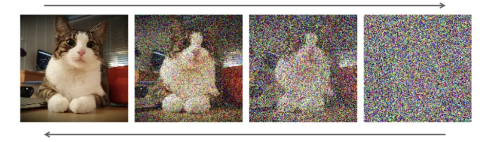
In the Forward process, we start with a real image and gradually add noise. As noise increases, the image becomes more and more blurry, eventually turning into white Gaussian noise.

In the Reverse process, we start with white noise and gradually remove noise through a neural network. As noise decreases, the image becomes clearer and clearer, eventually turning into a real image.

Prerequisites

Before diving into the math, let’s list the mathematical knowledge needed for the derivation.

Here, only the concept of “adding two Gaussian distributions” is needed:

The result of adding two Gaussian distributions is still a Gaussian distribution. Let the two Gaussian distributions be $\mathcal{N}(0, \sigma_a^2)$ and $\mathcal{N}(0, \sigma_b^2)$, then:

$$ \mathcal{N}(0,\sigma_a^2) + \mathcal{N}(0, \sigma_b^2) = \mathcal{N}(0, \sigma_a^2+\sigma_b^2) $$

This formula will be used in the Forward Process of the Diffusion Model.

Forward Process

The Forward Process is also called the “Diffusion Process.” Let the original image be $x_0$, and we gradually add noise to get $x_1, x_2, ..., x_t$. Eventually, $x_t$ will become white Gaussian noise.

$$ x_t = x_{t-1} + \epsilon_{t}, \quad \epsilon_{t} \sim \mathcal{N}(0, \bf{I}) $$

However, adding noise this straightforwardly might take forever to become pure white noise.

We want to get white Gaussian noise in a fixed number of steps $t$. The Diffusion Model adds noise using the following formula:

$$ x_t = \sqrt{\alpha_t} x_{t-1} + \sqrt{1-\alpha_t} \epsilon_{t}, \quad \epsilon_{t} \sim \mathcal{N}(0, \bf{I}) $$

Where $a_1, a_2, ... a_t$ are coefficients less than 1.

In each step of adding noise, besides adding Gaussian noise, the original image is also multiplied by a coefficient to weaken it, making the image’s original content less and less significant, and the Gaussian noise more and more dominant. By the $t$-th step, it can be fairly certain to become white Gaussian noise.

Starting from $x_0$, let’s go through the process of adding noise:

$$ \begin{align} x_1 &= \sqrt{\alpha_1}x_0 + \sqrt{1-\alpha_1}\epsilon_1 &\text{; where}\quad \epsilon_1, \epsilon_2..\epsilon_t \sim \mathcal{N}(0, \textbf{I}) \\ x_2 &= \sqrt{\alpha_2} x_1 + \sqrt{1-\alpha_2}\epsilon_2 \\ &= \sqrt{\alpha_2}(\sqrt{\alpha_1}x_0 + \sqrt{1-\alpha_1}\epsilon_1 ) + \sqrt{1-\alpha_2}\epsilon_2 \\ &= \sqrt{\alpha_1 \alpha_2 } x_0 + \textcolor{red}{\sqrt{\alpha_2 - \alpha_1\alpha_2} \epsilon_1 + \sqrt{1-\alpha_2}\epsilon_2} \\ &= \sqrt{\alpha_1 \alpha_2 } x_0 + \textcolor{red}{\sqrt{1 - \alpha_2 + \alpha_2 - \alpha_1\alpha_2} \overline{\epsilon}_2} \\ &= \sqrt{\alpha_1 \alpha_2 } x_0 + \sqrt{1 - \alpha_1\alpha_2} \overline{\epsilon_2} \\ x_3 &= \sqrt{\alpha_1\alpha_2\alpha_3} x_2 + \sqrt{1-\alpha_1\alpha_2\alpha_3}\overline{\epsilon}_3 \\ x_4 &= ... \\ x_t &= \sqrt{a_1..a_{t}} x_0 + \sqrt{1-\alpha_1...\alpha_{t}} \overline{\epsilon}_{t} \\ &= \sqrt{\overline{a_{t}}} x_0 + \sqrt{1-\overline{\alpha}_{t}} \overline{\epsilon}_{t} &\text{; where} \quad &\overline{a}_{t-1} = \prod_{t=1}^{T} a_{t} \ \\ \end{align} $$

It’s easy to see that $\overline{a}_{t}$ gets multiplied by a bunch of coefficients $<1$ and eventually gets close to 0, and $x_t$ will get infinitely close to $\overline{\epsilon}_t$ itself, which is just white noise from a Gaussian distribution.

With this equation, when training our neural network, we don’t need to loop through $t$ steps to add noise. Just plug in $x_0$ and $t$ into this equation, follow the agreed $\alpha$ sequence, and you can directly get the value $x_t$ after adding noise for the $t$-th step.

The magical part of this derivation is from $(4)$ to $(5)$.

$\sqrt{\alpha_2 - \alpha_1\alpha_2}\epsilon_1$ and $\sqrt{1-\alpha_2}\epsilon_2$ can be seen as a Reparameterization Trick, where they are samples from the normal distributions $\mathcal{N}(0, \alpha_2 - \alpha_1\alpha_2)$ and $\mathcal{N}(0, 1-\alpha_2)$ respectively.

Plugging these into the previous equation for adding two Gaussian distributions, we get:

$$ \mathcal{N}(0, \alpha_2 - \alpha_1\alpha_2) + \mathcal{N}(0, 1-\alpha_2) = \mathcal{N}(0, 1 - \alpha_1\alpha_2) $$

Which means:

$$ \sqrt{\alpha_2 - \alpha_1\alpha_2}\epsilon_1 + \sqrt{1-\alpha_2}\epsilon_2 = \sqrt{1 - \alpha_1\alpha_2} \overline{\epsilon}_2 \quad \text{; where} \quad \overline{\epsilon}_2 \sim \mathcal{N}(0, 1) $$

Backward Process

In the Forward Process, we start from $x_0$ and gradually add noise to get to $x_t$. In the Reverse Process, we use a denoising neural network to gradually remove noise $\overline{\epsilon}_t$ from $x_t$ to eventually get $x_0$.

A straightforward way to think about it is that we use the neural network to predict noise, and the goal of training the network is to make the predicted noise as close as possible to the actual noise:

$$ \begin{align} \mathcal{L} &= || \overline{\epsilon}_t - \epsilon_\theta(x_t, t) ||^2 \\ &= || \overline{\epsilon}_t - \epsilon_\theta(\sqrt{\overline{a}_t}x_0 + \sqrt{1-\overline{\alpha}_t}\overline{\epsilon}_t, t) ||^2 \\ \end{align} $$

Here, $\epsilon_\theta$ is our neural network, which takes $x_t$ and the current step $t$ as input and outputs the predicted noise.

This is just like the loss function at the end of the original Diffusion Model paper.

However, looking at this loss function, the goal of the denoising neural network is to optimize the sum of all noises from step $0$ to $t$, not just the noise at step $t$ alone. If you train it too hard, it might remove all noise in one go, right? But in practice, with enough training data, I guess the model can still generalize to gradually remove noise under this optimization goal. And judging by the current results, it seems to be working.

Training

Now, let’s put together the training process:

1. Sample an image from the training set as $x_0$
2. Randomly sample a $t$, calculate $x_t$ and noise $\overline{\epsilon}_t$ according to the agreed $\alpha$ sequence
3. Use $x_t$ and $t$ as input, predict noise $\epsilon_\theta(x_t, t)$ with the neural network, and calculate the loss with the actual noise $\overline{\epsilon}_t$
4. Get the gradients, update the neural network parameters
5. Go back to step 1 for the next round of training

Conclusion

The logic behind training Diffusion Models isn’t complicated. You add noise here, use a neural network to predict noise there, that’s it. The counterintuitive part is that the optimization goal for the Reverse Process isn’t just the noise at step $t$, but the total noise from step $0$ to $t$.

The ELBO part of the derivation is still tough for me, I’ll record that separately when I have time. My understanding is that the ELBO series of derivations serve as a proof of correctness, but in practice, the Diffusion Model doesn’t fully follow this mathematically optimal equation. Instead, it simplifies it a bit and finds better results through experiments, which are the most important.