In the last blog, I went over the intuition behind VAE, which was pretty straightforward. However, when reading articles about the math behind VAE, I always felt something was missing. So, I spent two weeks (except for eating and sleeping) working through the math until I finally got the formulas down. The whole process was quite challenging for someone with my math background, so I’m documenting it here.
Prerequisites
Before diving into the formulas, let’s review/preview the math we’ll be using. This way, we can just plug it in later.
Expected Value of Probability
Let’s quickly recall the concept of “expected value” in probability using a lottery example: Suppose there are two prizes in a lottery, first prize and second prize. The probability of winning first prize is 1%, with a reward of 10,000, and the probability of winning second prize is 10%, with a reward of 100. What is the expected value of the reward if I participate in this lottery?
$$ \mathbb{E}[x] = \sum_{i=1}^{n} x_i p_i(x_i) $$Here, $x$ is the random variable, $x_i$ corresponds to the reward for different prizes, and $p_i(x_i)$ is the probability for each prize. In this example, the expected reward is $10000 \times 0.01 + 100 \times 0.1 = 110$.
For continuous random variables, the expected value is calculated as:
$$ \mathbb{E}[x] = \int x p(x) dx $$The expected value can also be estimated using sampling. For example, if we have a sample set $X = \{x_1, x_2, \ldots, x_n\}$, the expected value can be estimated as:
$$ \mathbb{E}[x] \approx \frac{1}{n} \sum_{i=1}^{n} x_i, \,\,\,\, x_i \sim p(x) $$In our derivations, we can use this conversion to turn continuous expected values into discrete calculations using sampling:
$$ \begin{align*} \mathbb{E}[x] &= \int x p(x) dx \\ &\approx \frac{1}{n} \sum_{i=1}^{n} x_i, \,\,\,\, x_i \sim p(x) \end{align*} $$A typical sampling calculation is during a training round in machine learning, where we have a batch of training data. We can use this data as a sample set to estimate the expected value.
The expected value can also be applied to functions:
$$ \begin{align*} \mathbb{E}[f(x)] &= \int f(x) p(x) dx \\ &\approx \frac{1}{n} \sum_{i=1}^{n} f(x_i), \,\,\,\, x_i \sim p(x) \end{align*} $$The function usually used here is $\ln$. When the probability distribution is normal, substituting the normal distribution formula can lead to the least squares method, which connects to the loss functions we commonly see. We’ll see this process in detail later in our derivations.
Normal Distribution
The normal distribution, also known as the Gaussian distribution, is the bell curve we often talk about:
$$ \mathcal{N}(\mu, \sigma^2) = \frac{1}{\sqrt{2\pi\sigma^2}} \exp\left(-\frac{(x - \mu)^2}{2\sigma^2}\right) $$If human height follows a normal distribution, we can use this formula to calculate the probability of someone being 1.8 meters tall.
In VAE, the latent variables, encoder, and generator outputs are all set to follow a normal distribution. The normal distribution formula is used in their derivations.
KL Divergence
KL divergence measures the difference between two probability distributions and is defined as:
$$ \text{KL}(p||q) = \int p(x) \log \frac{p(x)}{q(x)} dx $$A property of KL divergence is that it is always greater than zero, which is used when calculating the ELBO as a lower bound.
According to Su’s blog, KL divergence is not the only way to measure the difference between two probability distributions, but it can be written in the form of an expected value, which is convenient in VAE derivations.
When comparing the KL divergence of two normal distributions, you can directly use the following formula:
$$ \begin{align*} \text{KL}(P || Q) &= \text{KL}(\mathcal{N}(\mu_P, \sigma_P^2) || \mathcal{N}(\mu_Q, \sigma_Q^2)) \\ &= \frac{1}{2} \left( \log \frac{\sigma_Q}{\sigma_P} + \frac{\sigma_P^2 + (\mu_P - \mu_Q)^2}{\sigma_Q^2} - 1 \right) \end{align*} $$When comparing to the standard normal distribution $\mathcal{N}(0,1)$, where $\mu_Q = 0$ and $\sigma_Q = 1$, it can be further simplified to:
Okay, here’s the translated Markdown:
$$ \text{KL}(\mathcal{N}(\mu_P, \sigma_P^2) || \mathcal{N}(0, 1)) = - \log \sigma_P + \frac{\sigma_P^2 + \mu_P^2 - 1}{2} $$Bayes’ Formula
Bayes’ formula tells us how to update our beliefs about events (like whether an image is a legit cat or dog pic) based on new evidence (like training data with cat and dog images):
$$ p(z|x) = \frac{p(x|z)p(z)}{p(x)} $$In the derivation of VAE, we plug in Bayes’ formula to calculate the conditional probability between latent variables and normal images.
Image Generation Model
From a probabilistic perspective, we assume the probability distribution $p(x)$ is the distribution of the images we want to generate.
How do we understand this probability distribution? We can think of $x$ as a vector of $128 \times 128$ pixels. For a valid image (like a cat or dog photo), $p(x)$ will be close to 1. For an invalid scrambled image, $p(x)$ will be close to 0.
The process of generating an image is like sampling from the $p(x)$ distribution.
But $x$ as a high-dimensional random variable, most possible values are invalid. We don’t know the exact form of $p(x)$, so we don’t know how to sample from it.
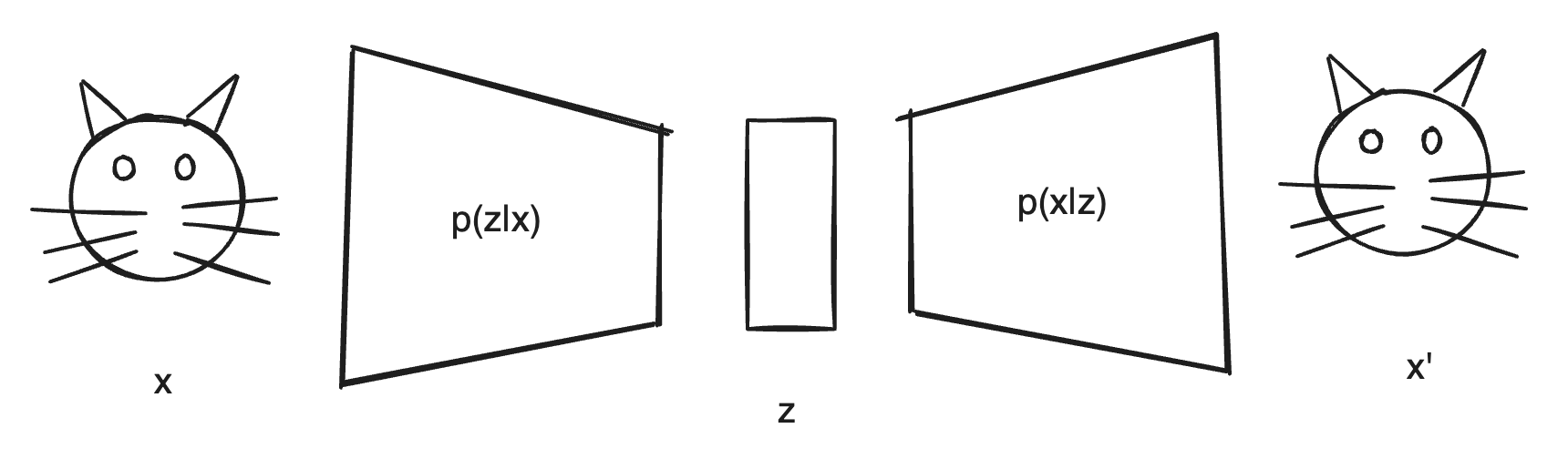
To solve the sampling problem, VAE introduces a latent variable $z$. When generating images, we first sample from a normal distribution $p(z)$, then sample $x$ from $p(x|z)$ to make $p(x)$ as close to 1 as possible.
This way, each sample always generates a valid image. $p(x|z)$ is also called the decoder.
As for $z$, it can be seen as an encoding of the original image. The encoder samples $z$ from $p(z|x)$ according to a normal distribution, resulting in a specific $z$.
During training, we want to maximize $p(x)$ using the training dataset $x$, so we learn a good encoder and decoder at the same time. When generating images, we only use the decoder.
From Maximizing $p(x)$ to ELBO
Since calculating $p(x)$ directly is very difficult, VAE introduces the idea of variational inference: introduce an approximate posterior distribution $q(z|x)$ to approximate $p(z|x)$. We can think of this approximate posterior distribution $q(z|x)$ as a probability distribution fitted by a neural network. Although we don’t know the exact distribution of $p(z|x)$ beforehand, we can optimize $q(z|x)$ by maximizing $p(x)$ to make it close to the true $p(z|x)$.
The derivation of maximizing $p(x)$ is as follows:
$$ \begin{align} \max p(x) &= \max \ln p(x) \\ &= \max \ln p(x) \textcolor{blue}{\underset{=1}{\int q(z|x) \, dz}} \\ &= \max \int q(z|x) \ln p(x) \, dz \\ &= \max \int q(z|x) \ln \textcolor{blue}{\frac{ p(x|z) p(z) }{ p(z|x)}} \, dz \\ &= \max \int q(z|x) \ln \frac{p(x|z) p(z) \, \textcolor{blue}{q(z|x)}}{p(z|x) \textcolor{blue}{q(z|x)}} \, dz \\ &= \max \underbrace{\int q(z|x) \ln \frac{q(z|x)}{p(z|x)} \, dz}_{KL \, Divergence} + \int q(z|x) \ln \frac{p(x|z)p(z)}{q(z|x)} dz \\ &= \max \underbrace{D_{KL} ( q((z|x) || p(z|x))}_{always\, \ge 0} + \int q(z|x) \ln \frac{p(x|z)p(z)}{q(z|x)} dz \\ &\ge \max \underbrace{\int q(z|x) \ln \frac{p(x|z)p(z)}{q(z|x)} dz}_{ELBO} \end{align} $$In $(2)$ and $(3)$, we plug in $\int q(z|x) dz$ which equals 1.
In $(4)$, we plug in Bayes’ formula, transforming $p(x)$ to $\frac{p(x|z) p(z)}{p(z|x)}$.
In $(5)$, we multiply by $\frac{q(z|x)}{q(z|x)}$ which equals 1, and in $(5)$ we can get the KL divergence between $q(z|x)$ and $p(z|x)$.
Using the property that KL divergence is always greater than zero, we can get the lower bound of $\ln p(x)$, which is ELBO.
$$ ELBO = \int q(z|x) \ln \frac{p(x|z)p(z)}{q(z|x)} dz $$$p(x)$ is always greater than ELBO, so we can maximize $p(x)$ by maximizing ELBO.
From ELBO to Training Objectives
The ELBO formula can’t be used directly for training models, so let’s derive it further:
$$ \begin{align} ELBO &= \int q(z|x) \ln \frac{p(x|z)p(z)}{q(z|x)} dz \\ &= \int q(z|x) \ln \frac{p(z)}{q(z|x)} dz + \int q(z|x) \ln p(x|z) dz \\ &= - \int q(z|x) \ln \frac{q(z|x)}{p(z)} dz + \int q(z|x) \ln p(x|z) dz \\ &= - D_{KL}(q(z|x) || p(z)) + \mathbb{E}_{z \sim q(z|x)}[\ln p(x|z)] \end{align} $$When used as a loss function, we usually prefer to minimize it, so we can take the negative of ELBO to get the Loss function:
$$ \mathcal{L} = - ELBO = D_{KL}(q(z|x) || p(z)) - \mathbb{E}_{z \sim q(z|x)}[\ln p(x|z)] $$The key part of the derivation seems to be the KL divergence between $q(z|x)$ and $p(z)$, corresponding to the “Divergence Loss”; the rest is the expectation of $\ln p(x|z)$ under $q(z|x)$, corresponding to the “Reconstruct Loss,” which matches the two parts of the loss function from the previous article.
Substituting Normal Distributions
Earlier, we mentioned that $p(z)$, $q(z|x)$, and $p(x|z)$ are all normal distributions. We know that $p(z)$ is a standard normal distribution $\mathcal{N}(0, 1)$, and both $q(z|x)$ and $p(x|z)$ come from neural network fitting.
Let the parameters of $q(z|x)$ and $p(x|z)$ be $\theta$ and $\phi$, respectively:
$$ \begin{align*} q_\theta(z|x) &= \mathcal{N}(\mu_\theta(x), \sigma_\theta(x)^2) \\ p_\phi(x|z) &= \mathcal{N}(\mu_\phi(z), \sigma_\phi(z)^2) \end{align*} $$First, let’s look at the Divergence Loss part, which can be substituted into the formula for calculating the KL divergence with the standard normal distribution $\mathcal{N}(0,1)$:
$$ \begin{align*} \min_\theta \text{Divergence Loss} &= \min_\theta D_{KL}(q_\theta(z|x) || p(z)) \\ &= \min_\theta D_{KL}(\mathcal{N}(\mu_\theta(x), \sigma_\theta(x)^2) || \mathcal{N}(0, 1)) \\ &= \min_\theta - \ln \sigma_\theta(x) + \frac{\sigma_\theta(x)^2 + \mu_\theta(x)^2 - 1}{2} \end{align*} $$Here, $\sigma_\theta(x)$ and $\mu_\theta(x)$ come from the encoder’s output.
Next, let’s look at the Reconstruct Loss part, which can be substituted into the formula for calculating the expectation with the normal distribution $\mathcal{N}(\mu_\phi(z), \sigma_\phi(z)^2)$. In the decoder part, we can make $\sigma_\phi(z)$ always a fixed constant:
$$ \begin{align} \min_\phi \text{Reconstruct Loss} &= \max_\phi \mathbb{E}_{z \sim q(z|x)}[\ln p_\phi(x|z)] \\ &= \max_\phi \mathbb{E}_{z \sim q(z|x)}[\ln \mathcal{N}(\mu_\phi(z), \sigma_\phi(z)^2)] \\ &= \max_\phi \mathbb{E}_{z \sim q(z|x)}[\ln \frac{1}{\sqrt{2\pi} \sigma_\phi(z)} \exp(-\frac{(x - \mu_\phi(z))^2}{2\sigma_\phi(z)^2})] \\ &= \max_\phi \mathbb{E}_{z \sim q(z|x)}[-\ln \sqrt{2\pi} - \ln \sigma_\phi(z) - \frac{(x - \mu_\phi(z))^2}{2\sigma_\phi(z)^2}] \\ &\cong \max_\phi \sum_i^N [-\ln \sqrt{2\pi} - \ln \sigma_\phi(z_i) - \frac{(x_i - \mu_\phi(z_i))^2}{2\sigma_\phi(z_i)^2}] \\ &= \min_\phi \sum_i^N [\ln \sqrt{2\pi} + \ln \sigma_\phi(z_i) + \frac{(x_i - \mu_\phi(z_i))^2}{2\sigma_\phi(z_i)^2}] \\ &= \min_\phi \sum_i^N [\ln \sigma_\phi(z_i) + \frac{(x_i - \mu_\phi(z_i))^2}{2\sigma_\phi(z_i)^2}] \\ &= \min_\phi \sum_i^N {(x_i - \mu_\phi(z_i))^2} \end{align} $$In equation $(17)$, we replace the expected calculation with a sampled estimate, allowing the training set to be included in the calculation. Each sample of $z$ during training comes from the distribution of $q(z|x)$, which can be enumerated discretely during training.
In equation $(19)$, substituting $\sigma_\phi(z)$ as a constant, the final equation becomes equivalent to least squares, comparing each pixel of the generated image with the original image.
Final Thought
By now, the formulas we’ve derived are exactly the same as the loss function in the previous article. Optimizing ELBO serves two purposes: it makes the encoder’s output closer to a normal distribution and also makes the decoder’s generated images closer to the original images.
(However, I’m still not clear whether this derivation process came first with variational inference and then the loss function, or if the loss function was the arrow that was shot and then the derivation process was the target drawn backwards.)