Recently, I wanted to learn about Stable Diffusion, but it seemed like I needed to first understand what VAE (Variational Autoencoder) is all about. Here, I’ll jot down my naive understanding of VAE. I haven’t fully grasped the math behind ELBO yet, so I’ll note that separately later.

The article “Intuitively Understanding Variational Autoencoders” does a great job explaining the intuition behind VAE, so this is kind of a manual summary.

Autoencoder

Before diving into VAE, let’s visit the older Autoencoder model first:

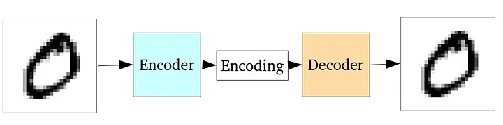
An Autoencoder consists of two neural networks: the left one is called the Encoder, which converts the input image into a low-dimensional Encoding vector (also known as the Latent vector). The right one is the Decoder, which takes the Encoding as input and reconstructs the original image.

It’s like a compression and decompression process.

The Encoding is much smaller than the original image. How can such a tiny Encoding vector reconstruct the complex original image?

When we learn to use neural networks for digit recognition, we have an intuition that some shallow neurons are good at recognizing “strokes,” while others are good at recognizing “crosses.” Each layer of the neural network extracts more advanced features, eventually corresponding to a 10-dimensional output.

This intuition can also help us understand how Autoencoders work: The Encoder’s neurons recognize “strokes,” “crosses,” “horizontal lines,” “vertical lines,” and other higher-level, intrinsic features, placing this information in the Encoding. The Decoder’s neurons learn how to use these “strokes,” “crosses,” “horizontal lines,” and “vertical lines” along with higher-level features to draw the image.

Since the Encoding vector’s dimensions are limited, the entire Autoencoder must learn to extract the most important features of the input image, inevitably making some trade-offs with the original information. In this way, the Encoder compresses the input data by learning the intrinsic structure and most important features of the data. With these features and the Decoder’s “drawing skills,” it can reconstruct the original image as closely as possible.

Training an Autoencoder is unsupervised; it doesn’t require data labeling. You can directly compare the original input with the Decoder’s final output for training. The loss function used in training is called “Reconstruction Loss,” which is simply calculated using MSE:

def ae_loss(input, output):
	# compute the average MSE error, then scale it up i.e. simply sum on all axes
	reconstruction_loss = sum(square(output-input))
	return reconstruction_loss

Limitations of Autoencoder

A well-trained Autoencoder has strong reconstruction capabilities, showing its strong drawing skills. However, its application scenarios are limited, only useful in a few places like image denoising.

What limits its potential? The problem lies in the Encoding vector being a black box: The Latent space of the Encoding vector is likely discrete and discontinuous.

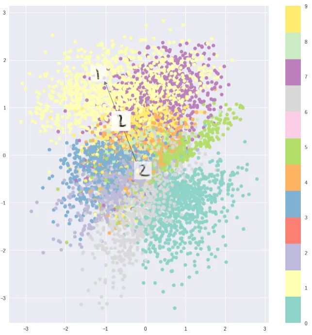
Typical Encodings show some clustering, but they are not continuous, making it impossible to arrange our requirements into the Encoding vector to guide the Autoencoder’s generation. Thus, it cannot be used as a generative model. If we randomly sample a vector from the latent space, it will most likely produce noise.

Ideally, the entire Latent space should be continuous, with typical Encodings (like those for digits 7 and 1) clustering. Sampling at the edges of these clusters should produce blurry “gradients” rather than noise:

Introducing Sampling

VAE solves this problem by making the Latent space fully continuous, allowing random sampling for generation and even connecting with text Embeddings for useful generation.

How do we make the Latent space continuous?

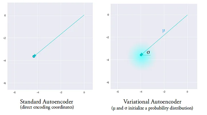
The first problem to solve is that in Autoencoders, each feature is point-like, and a slight deviation in position can lead the Decoder to draw completely different images.

VAE uses two vectors, $\mu$ and $\sigma$, to replace the point-like Encoding vector and adds a Sampling stage. $\mu$ and $\sigma$ correspond to the mean and standard deviation of a normal distribution, and Sampling involves sampling from this normal distribution.

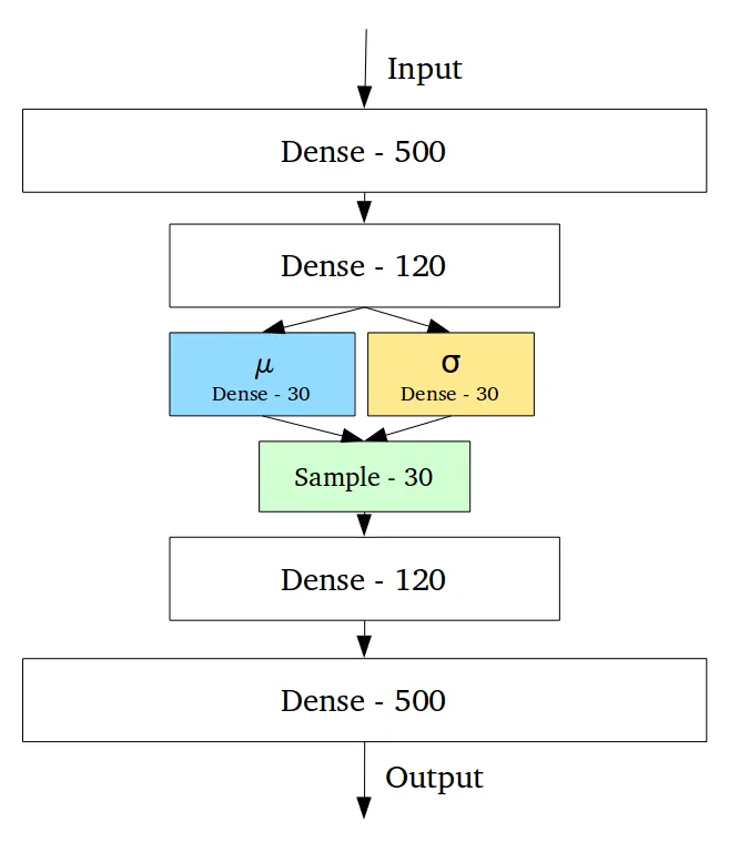
This way, during training, the Decoder can be less obsessed with pinpoint Encoding vectors and more flexible, reconstructing images within a sphere space centered at $\mu$ with a radius of $\sigma$.

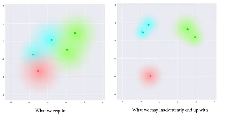
However, neural networks might still find sneaky shortcuts during training, leaving vast distances between different distributions in the Latent space:

KL Divergence

The idea of VAE to make the entire Latent space continuous is to make it as close as possible to a normal distribution $Normal(0, 1)$ with a mean of 0 and a standard deviation of 1.

KL Divergence (Kullback–Leibler divergence) can measure the difference between two probability distributions. The formula for comparing the KL divergence between two normal distributions is:

Substituting a normal distribution with a mean of 0 and a standard deviation of 1 as the other distribution to compare, the formula for calculating KL divergence for $\mu$ and $\sigma$ vectors is:

However, during training, we need to compare not just one normal distribution to $Normal(0, 1)$, but the total difference between N normal distributions and $Normal(0,1)$. It seems like summing all the KL divergence comparisons still reflects the overall difference from $Normal(0, 1)$. Some mathematical derivations might still be unclear, but we’ll figure it out later.

By including KL divergence in the loss function, it acts as a regularizer, resulting in this complete loss function:

def vae_loss(input_img, output, log_stddev, mean):
	# compute the average MSE error, then scale it up i.e. simply sum on all axes
	reconstruction_loss = sum(square(output-input_img))
	# compute the KL loss
	kl_loss = -0.5 * sum(1 + log_stddev - square(mean) - square(exp(log_stddev)), axis=-1)
	# return the average loss over all images in batch
	total_loss = mean(reconstruction_loss + kl_loss)
	return total_loss

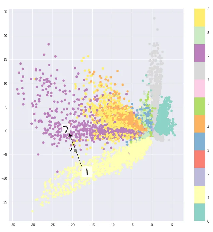
With KL divergence applied, the trained Latent space should be closer to the desired distribution shape: